knitr::opts_chunk$set(
echo = TRUE,
message = FALSE,
warning = FALSE
)

library(tidyverse)
library(readxl)
library(janitor)
library(ggplot2)
library(maps)
library(ggcorrplot)5 Florida Crime Analytics
5.1 Introduction
In this assignment, I acted as a data analyst for the Florida Police Department. I was tasked with discovering which economic factors were most strongly associated with rising crime rates across Florida counties. In particular, the FPD (Florida Police Department) was interest in the role of income, education, and urbanization in explaining these differences.
5.2 Loading and Preparing the Data
Florida <- read_xlsx("Florida County Crime Rates.xlsx")

FloridaRenamed <- Florida %>%
  rename(
Crime        = C,
Income         = I,
HighSchoolGrad = HS,
UrbanPop       = U
) %>%
  mutate(
    County = str_to_title(str_trim(County))
  )

glimpse(FloridaRenamed)
Rows: 67
Columns: 5
$ County <chr> "Alachua", "Baker", "Bay", "Bradford", "Brevard", "Brow…
$ Crime <dbl> 104, 20, 64, 50, 64, 94, 8, 35, 27, 41, 55, 69, 128, 69…
$ Income <dbl> 22.1, 25.8, 24.7, 24.6, 30.5, 30.6, 18.6, 25.7, 21.3, 3…
$ HighSchoolGrad <dbl> 82.7, 64.1, 74.7, 65.0, 82.3, 76.8, 55.9, 75.7, 68.6, 8…
$ UrbanPop <dbl> 73.2, 21.5, 85.0, 23.2, 91.9, 98.9, 0.0, 80.2, 31.0, 65…summary(FloridaRenamed) County Crime Income HighSchoolGrad
Length:67 Min. : 0.0 Min. :15.40 Min. :54.50
Class :character 1st Qu.: 35.5 1st Qu.:21.05 1st Qu.:62.45
Mode :character Median : 52.0 Median :24.60 Median :69.00
Mean : 52.4 Mean :24.51 Mean :69.49
3rd Qu.: 69.0 3rd Qu.:28.15 3rd Qu.:76.90
Max. :128.0 Max. :35.60 Max. :84.90
UrbanPop
Min. : 0.00
1st Qu.:21.60
Median :44.60
Mean :49.56
3rd Qu.:83.55
Max. :99.60 5.3 Exploratory Data Analysis
summary_stats <- FloridaRenamed %>%
  summarise(
    mean_crime = mean(Crime),
    median_crime = median(Crime),
    min_crime = min(Crime),
    max_crime = max(Crime),
    range_crime = max(Crime) - min(Crime),

    mean_income = mean(Income),
    median_income = median(Income),
    min_income = min(Income),
    max_income = max(Income),
    range_income = max(Income) - min(Income),

    mean_HS = mean(HighSchoolGrad),
    median_HS = median(HighSchoolGrad),
    min_HS = min(HighSchoolGrad),
    max_HS = max(HighSchoolGrad),
    range_HS = max(HighSchoolGrad) - min(HighSchoolGrad),

    mean_urban = mean(UrbanPop),
    median_urban = median(UrbanPop),
    min_urban = min(UrbanPop),
    max_urban = max(UrbanPop),
    range_urban = max(UrbanPop) - min(UrbanPop)
  )

knitr::kable(as.data.frame(t(summary_stats)))| V1 | |
|---|---|
| mean_crime | 52.40299 |
| median_crime | 52.00000 |
| min_crime | 0.00000 |
| max_crime | 128.00000 |
| range_crime | 128.00000 |
| mean_income | 24.51045 |
| median_income | 24.60000 |
| min_income | 15.40000 |
| max_income | 35.60000 |
| range_income | 20.20000 |
| mean_HS | 69.48955 |
| median_HS | 69.00000 |
| min_HS | 54.50000 |
| max_HS | 84.90000 |
| range_HS | 30.40000 |
| mean_urban | 49.55821 |
| median_urban | 44.60000 |
| min_urban | 0.00000 |
| max_urban | 99.60000 |
| range_urban | 99.60000 |
Grad_Income_Graph <- ggplot(FloridaRenamed, aes(x = HighSchoolGrad, y = Income)) +
  geom_point(color = "green") +
  geom_hline(yintercept = 0, linetype = "dashed") +
  geom_smooth(se = FALSE, color = "black", linetype = "solid")+
  labs(
    title = "How Graduation Rate Impacts Income",
    x = "High School Graduation Rate",
    y = "Income"
  )
print(Grad_Income_Graph)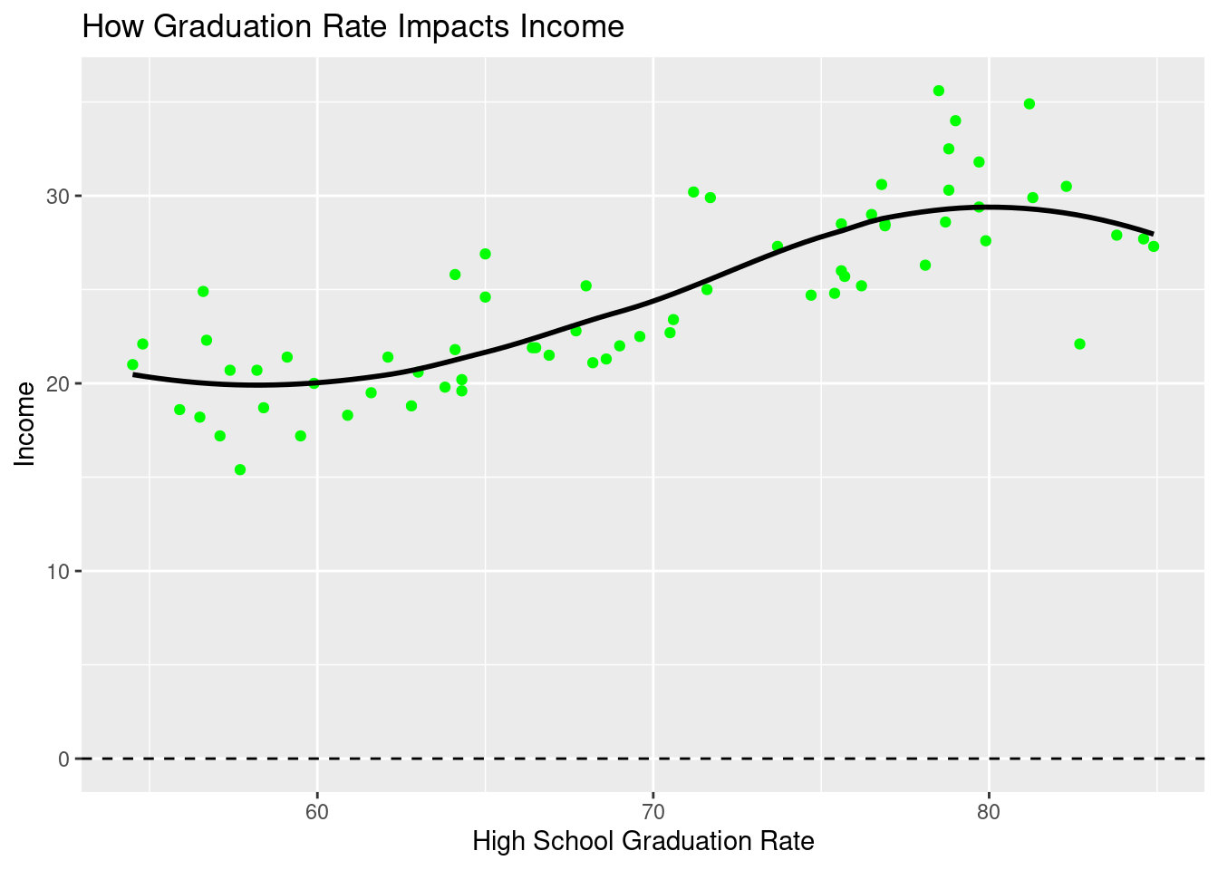
Note
Income appears to rise with high school graduation rates (though it appears relatively stable past 75%).
UrbanPop_Crime_graph <- ggplot(FloridaRenamed, aes(x = UrbanPop, y = Crime)) +
  geom_point() +
  geom_smooth(method = "lm", se=TRUE) +
  labs(
    title = "Crime vs Urban Population",
    x = "Urban Population",
    y = "Crime"
  ) +
  theme_minimal()

print(UrbanPop_Crime_graph)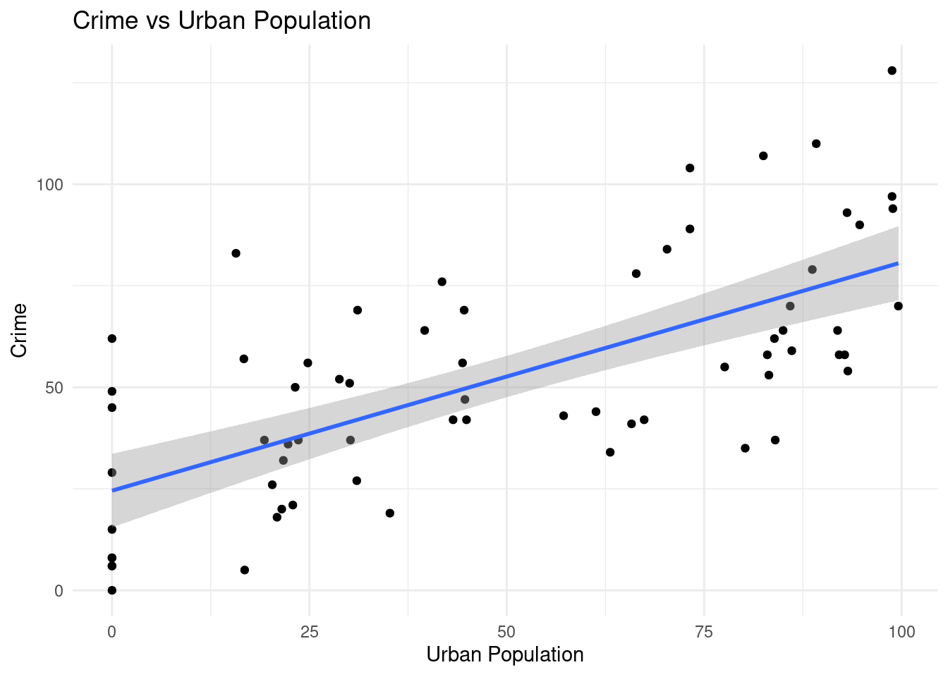
Crime appears to rise with urban population.
fl_map <- map_data("county") %>%
  filter(region == "florida") %>%
  mutate(subregion = str_to_title(subregion))


fl_map_data <- fl_map %>%
  left_join(FloridaRenamed %>% rename(subregion = County),
            by = "subregion")


ggplot(fl_map_data, aes(long, lat, group = group, fill = Crime)) +
  geom_polygon(color = "white", linewidth = 0.2) +
  coord_quickmap() +
  scale_fill_gradient(low = "lemonchiffon", high = "red", na.value = "grey90") +
  labs(
    title = "Florida Counties: Crime Rate",
    fill  = "Crime Rate"
  ) +
  theme_void()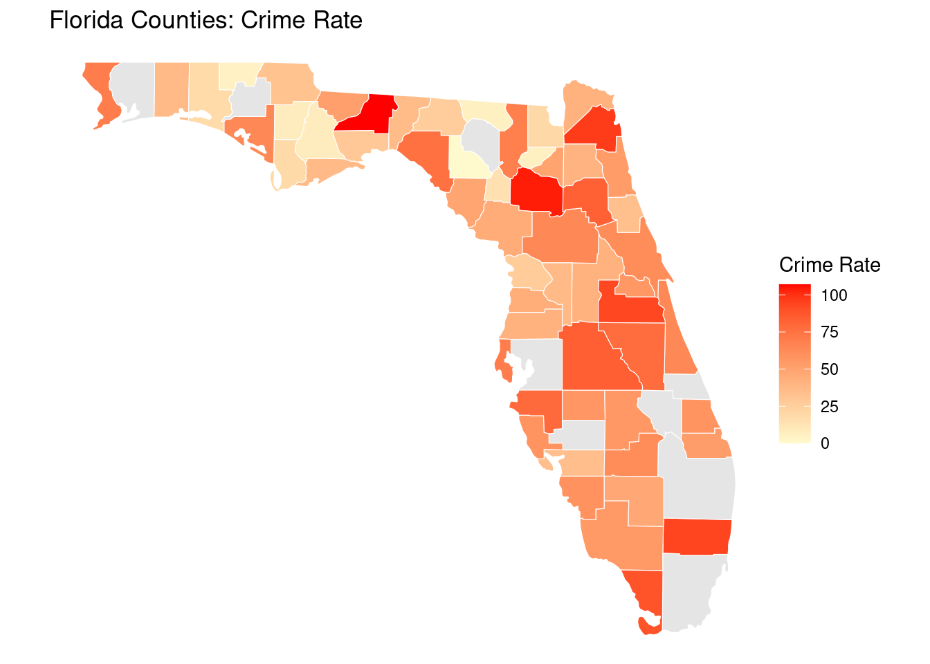
5.4 Correlation Analysis
cor_data <- FloridaRenamed[, c("Crime", "Income", "HighSchoolGrad", "UrbanPop")]
cor_matrix <- cor(cor_data, use = "complete.obs")
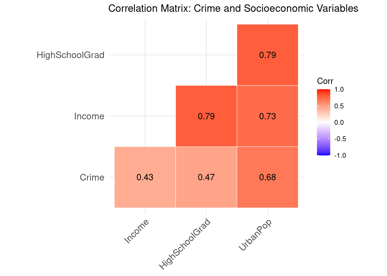
cor_matrix Crime Income HighSchoolGrad UrbanPop
Crime 1.0000000 0.4337503 0.4669119 0.6773678
Income 0.4337503 1.0000000 0.7926215 0.7306983
HighSchoolGrad 0.4669119 0.7926215 1.0000000 0.7907190
UrbanPop 0.6773678 0.7306983 0.7907190 1.0000000Urban population shows the highest correlation with crime. This is a strong correlation. All the correlations are positive. Some, such as “Crime/UrbanPop”,“Income/HighSchoolGrad”, “Income/UrbanPop”, “HighSchoolGrad/UrbanPop”, are strong. The others are all moderate.
ggcorrplot(
  cor_matrix,
  lab = TRUE,
  lab_size = 4,
  method = "square",
  type = "lower",
  outline.col = "white",
  title = "Correlation Matrix: Crime and Socioeconomic Variables"
)
5.5 Building Regression Models
simplecrimemodel <- lm(Crime ~ UrbanPop, data = FloridaRenamed)

summary(simplecrimemodel)
Call:
lm(formula = Crime ~ UrbanPop, data = FloridaRenamed)

Residuals:
    Min      1Q  Median      3Q     Max
-34.766 -16.541  -4.741  16.521  49.632

Coefficients:
            Estimate Std. Error t value Pr(>|t|)
(Intercept) 24.54125    4.53930   5.406 9.85e-07 ***
UrbanPop     0.56220    0.07573   7.424 3.08e-10 ***
---
Signif. codes:  0 '***' 0.001 '**' 0.01 '*' 0.05 '.' 0.1 ' ' 1

Residual standard error: 20.9 on 65 degrees of freedom
Multiple R-squared:  0.4588,    Adjusted R-squared:  0.4505
F-statistic: 55.11 on 1 and 65 DF, p-value: 3.084e-10Twowaycrimemodel <- lm(Crime ~ UrbanPop + Income, data = FloridaRenamed)
summary(Twowaycrimemodel)
Call:
lm(formula = Crime ~ UrbanPop + Income, data = FloridaRenamed)

Residuals:
    Min      1Q  Median      3Q     Max
-36.130 -15.590  -6.484  16.595  48.921

Coefficients:
            Estimate Std. Error t value Pr(>|t|)
(Intercept)  39.9723    16.3536   2.444   0.0173 *
UrbanPop      0.6418     0.1110   5.784 2.36e-07 ***
Income       -0.7906     0.8049  -0.982   0.3297
---
Signif. codes:  0 '***' 0.001 '**' 0.01 '*' 0.05 '.' 0.1 ' ' 1

Residual standard error: 20.91 on 64 degrees of freedom
Multiple R-squared:  0.4669,    Adjusted R-squared:  0.4502
F-statistic: 28.02 on 2 and 64 DF, p-value: 1.815e-09Fullcrimemodel <- lm(Crime ~ UrbanPop + Income + HighSchoolGrad, data=FloridaRenamed)
summary(Fullcrimemodel)
Call:
lm(formula = Crime ~ UrbanPop + Income + HighSchoolGrad, data = FloridaRenamed)

Residuals:
    Min      1Q  Median      3Q     Max
-35.407 -15.080  -6.588  16.178  50.125

Coefficients:
               Estimate Std. Error t value Pr(>|t|)
(Intercept)     59.7147    28.5895   2.089   0.0408 *
UrbanPop         0.6972     0.1291   5.399 1.08e-06 ***
Income          -0.3831     0.9405  -0.407   0.6852
HighSchoolGrad  -0.4673     0.5544  -0.843   0.4025
---
Signif. codes:  0 '***' 0.001 '**' 0.01 '*' 0.05 '.' 0.1 ' ' 1

Residual standard error: 20.95 on 63 degrees of freedom
Multiple R-squared:  0.4728,    Adjusted R-squared:  0.4477
F-statistic: 18.83 on 3 and 63 DF, p-value: 7.823e-09AIC(simplecrimemodel,Twowaycrimemodel,Fullcrimemodel) df AIC
simplecrimemodel 3 601.4300
Twowaycrimemodel 4 602.4276
Fullcrimemodel 5 603.6764The simple crime model and two way crime model are effectively the same when it comes to AIC. So, the simple crime model is likely the best (being that it involves the fewest different variables). The simple model explains about 46% of the variance in crime (Adjusted R² ≈ 0.45), which is only slightly lower than the other models. Because it explains a similar amount of variance while using the fewest predictors, the simple crime model is the most parsimonious. In addition, the other variables are not significant when urban population is included in the model (p > .05 for both high school graduation and income). It is, therefore, relatively clear that urban population is the strongest predictor of crime. This makes intuitive sense: The more people in a given area, the more people there are who are capable of committing crimes.
5.6 Communicate Your Findings
The best model for predicting crime is the “simple crime model.” It explains the same amount of variance as the other models, has the lowest AIC, and is the most parsimonious (being that it only includes one variable). As a result, the Florida PD should invest more resources in more populated areas.
A limitation of this analysis is that factors which result from large population (such as crowded living conditions or food scarcity) may be at the heart of crime issues. It may be more effective to address these issues directly than to simply put more resources into more populated areas. If this is the case, the simple crime model is not wrong (per se) — it is merely too broad. A future analysis should explore which variables associated with large population may or may not be at the root of crime.